50-lines multi-xPU example

This concise multi-xPU 3-D heat diffusion solver uses ParallelStencil in conjunction with ImplicitGlobalGrid.jl and can be readily deployed on a single CPU thread or on thousands of GPUs/CPUs. Again, a simple boolean USE_GPU defines whether it runs on GPU(s) or CPU(s). The solver can be run with any number of processes. ImplicitGlobalGrid.jl creates automatically an implicit global computational grid based on the number of processes the solver is run with (and based on the process topology, which can be explicitly chosen by the user or automatically determined). Please refer to the documentation of ImplicitGlobalGrid.jl for more information.

julia

const USE_GPU = true
using ImplicitGlobalGrid
import MPI
using ParallelStencil
using ParallelStencil.FiniteDifferences3D
@static if USE_GPU
    @init_parallel_stencil(CUDA, Float64, 3);
else
    @init_parallel_stencil(Threads, Float64, 3);
end

@parallel function diffusion3D_step!(T2, T, Ci, lam, dt, dx, dy, dz)
    @inn(T2) = @inn(T) + dt*(lam*@inn(Ci)*(@d2_xi(T)/dx^2 + @d2_yi(T)/dy^2 + @d2_zi(T)/dz^2));
    return
end

function diffusion3D()
# Physics
lam        = 1.0;                                        # Thermal conductivity
cp_min     = 1.0;                                        # Minimal heat capacity
lx, ly, lz = 10.0, 10.0, 10.0;                           # Length of computational domain in dimension x, y and z

# Numerics
nx, ny, nz = 256, 256, 256;                              # Number of gridpoints in dimensions x, y and z
nt         = 100;                                        # Number of time steps
init_global_grid(nx, ny, nz);
dx         = lx/(nx_g()-1);                              # Space step in x-dimension
dy         = ly/(ny_g()-1);                              # Space step in y-dimension
dz         = lz/(nz_g()-1);                              # Space step in z-dimension

# Array initializations
T   = @zeros(nx, ny, nz);
T2  = @zeros(nx, ny, nz);
Ci  = @zeros(nx, ny, nz);

# Initial conditions (heat capacity and temperature with two Gaussian anomalies each)
Ci .= 1.0./( cp_min .+ Data.Array([5*exp(-((x_g(ix,dx,Ci)-lx/1.5))^2-((y_g(iy,dy,Ci)-ly/2))^2-((z_g(iz,dz,Ci)-lz/1.5))^2) +
                                   5*exp(-((x_g(ix,dx,Ci)-lx/3.0))^2-((y_g(iy,dy,Ci)-ly/2))^2-((z_g(iz,dz,Ci)-lz/1.5))^2) for ix=1:size(T,1), iy=1:size(T,2), iz=1:size(T,3)]) )
T  .= Data.Array([100*exp(-((x_g(ix,dx,T)-lx/2)/2)^2-((y_g(iy,dy,T)-ly/2)/2)^2-((z_g(iz,dz,T)-lz/3.0)/2)^2) +
                   50*exp(-((x_g(ix,dx,T)-lx/2)/2)^2-((y_g(iy,dy,T)-ly/2)/2)^2-((z_g(iz,dz,T)-lz/1.5)/2)^2) for ix=1:size(T,1), iy=1:size(T,2), iz=1:size(T,3)])
T2 .= T;                                                 # Assign also T2 to get correct boundary conditions.

# Time loop
dt = min(dx^2,dy^2,dz^2)*cp_min/lam/8.1;                 # Time step for the 3D Heat diffusion
for it = 1:nt
    @parallel diffusion3D_step!(T2, T, Ci, lam, dt, dx, dy, dz);
    update_halo!(T2);
    T, T2 = T2, T;
end

finalize_global_grid();
end

diffusion3D()

The corresponding file can be found here.

Thanks to ImplicitGlobalGrid.jl, only a few function calls had to be added in order to turn the single GPU/CPU solver into a multi-xPU solver (omitted unmodified lines are represented with #(...)):

julia

#(...)
using ImplicitGlobalGrid
#(...)
function diffusion3D()
# Physics
#(...)
# Numerics
#(...)
init_global_grid(nx, ny, nz);
dx  = lx/(nx_g()-1);                                     # Space step in x-dimension
dy  = ly/(ny_g()-1);                                     # Space step in y-dimension
dz  = lz/(nz_g()-1);                                     # Space step in z-dimension

# Array initializations
#(...)

# Initial conditions (heat capacity and temperature with two Gaussian anomalies each)
Ci .= 1.0./( cp_min .+ Data.Array([5*exp(-((x_g(ix,dx,Ci)-lx/1.5))^2-((y_g(iy,dy,Ci)-ly/2))^2-((z_g(iz,dz,Ci)-lz/1.5))^2) +
                                   5*exp(-((x_g(ix,dx,Ci)-lx/3.0))^2-((y_g(iy,dy,Ci)-ly/2))^2-((z_g(iz,dz,Ci)-lz/1.5))^2) for ix=1:size(T,1), iy=1:size(T,2), iz=1:size(T,3)]) )
T  .= Data.Array([100*exp(-((x_g(ix,dx,T)-lx/2)/2)^2-((y_g(iy,dy,T)-ly/2)/2)^2-((z_g(iz,dz,T)-lz/3.0)/2)^2) +
                   50*exp(-((x_g(ix,dx,T)-lx/2)/2)^2-((y_g(iy,dy,T)-ly/2)/2)^2-((z_g(iz,dz,T)-lz/1.5)/2)^2) for ix=1:size(T,1), iy=1:size(T,2), iz=1:size(T,3)])

# Time loop
#(...)
for it = 1:nt
    #(...)
    update_halo!(T2);
    #(...)
end

finalize_global_grid();
end

diffusion3D()

Here is the resulting movie when running the application on 8 GPUs, solving 3-D heat diffusion with heterogeneous heat capacity (two Gaussian anomalies) on a global computational grid of size 510x510x510 grid points. It shows the x-z-dimension plane in the middle of the dimension y: 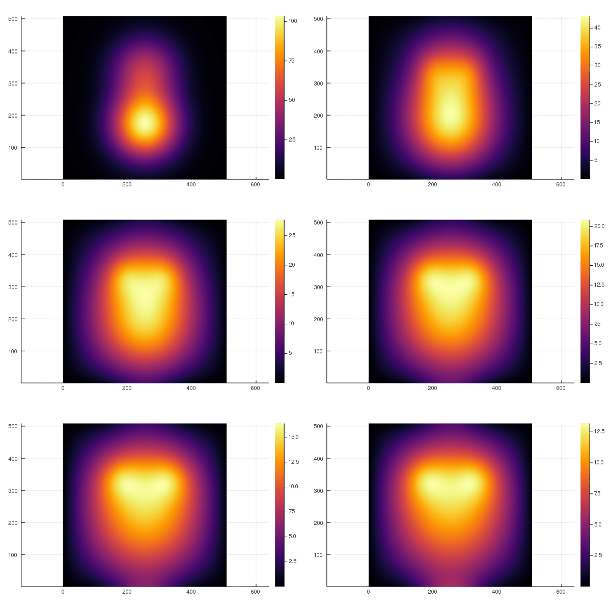3-D heat diffusion on 8 GPUs

The corresponding file, which also hides the communication behind computation with @hide_communication, can be found here.

50-lines multi-xPU example ​

50-lines multi-xPU example